If you’re here from the QR code — welcome. The poster gave you the summary. This page shows the method working.
The core intuition: jolts
The poster mentions HiPPO representations, but doesn’t have room to explain why they’re useful for anomaly detection. Here’s the idea.
HiPPO continuously compresses a stream of observations into a compact coefficient vector — essentially a polynomial approximation of the recent history of the signal. When something unexpected happens — a sudden offset, a spike, a slow drift — the update to that coefficient vector is abruptly large. We call these jolts.
The figure below shows this on a synthetic signal with two induced changes: a step offset at t = 2000 and a slow baseline drift beginning at t = 4000. The top panel is the raw signal, the middle panel shows the HiPPO state coefficients evolving over time (note how the first coefficient tracks the baseline, and higher-order coefficients respond to finer structure), and the bottom panel shows the magnitude of state updates — the jolts are clearly visible at both change-points.
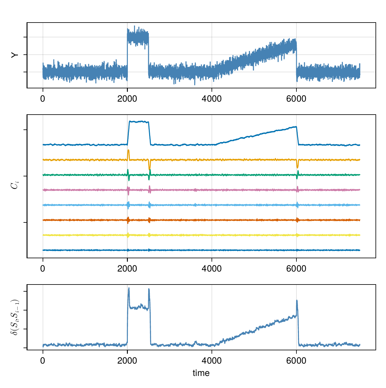
This is the foundation of HiAD’s anomaly score: at each timestep, compute how large the state update was, and ask how likely that magnitude is given the history so far. The probability is estimated non-parametrically via an online kernel histogram — no assumptions about the distribution of distances, no training required.
Try it: live demo
The interactive demo below runs a simplified version of HiAD directly in your browser. A Gaussian noise signal streams continuously. You can inject three types of anomaly and watch the distance and score panels respond in real time. Adjust the parameters, then hit reset, to see how they affect sensitivity.
Show Document in new tab: hiad_interactive_demo.html
What to try:
- Hit inject offset and watch the distance spike immediately, followed by the score crossing the threshold (red dashed line)
- Hit inject drift — the score rises more gradually, reflecting the slower change
- Set β = 0 then inject an offset — notice the score stays elevated for much longer (the model rejects the anomalous data from its state entirely, causing cascading false positives on a drifting signal)
- Increase N (and reset) for a more expressive state representation; decrease it for faster, cruder detection
Speed vs. accuracy: the Pareto frontier
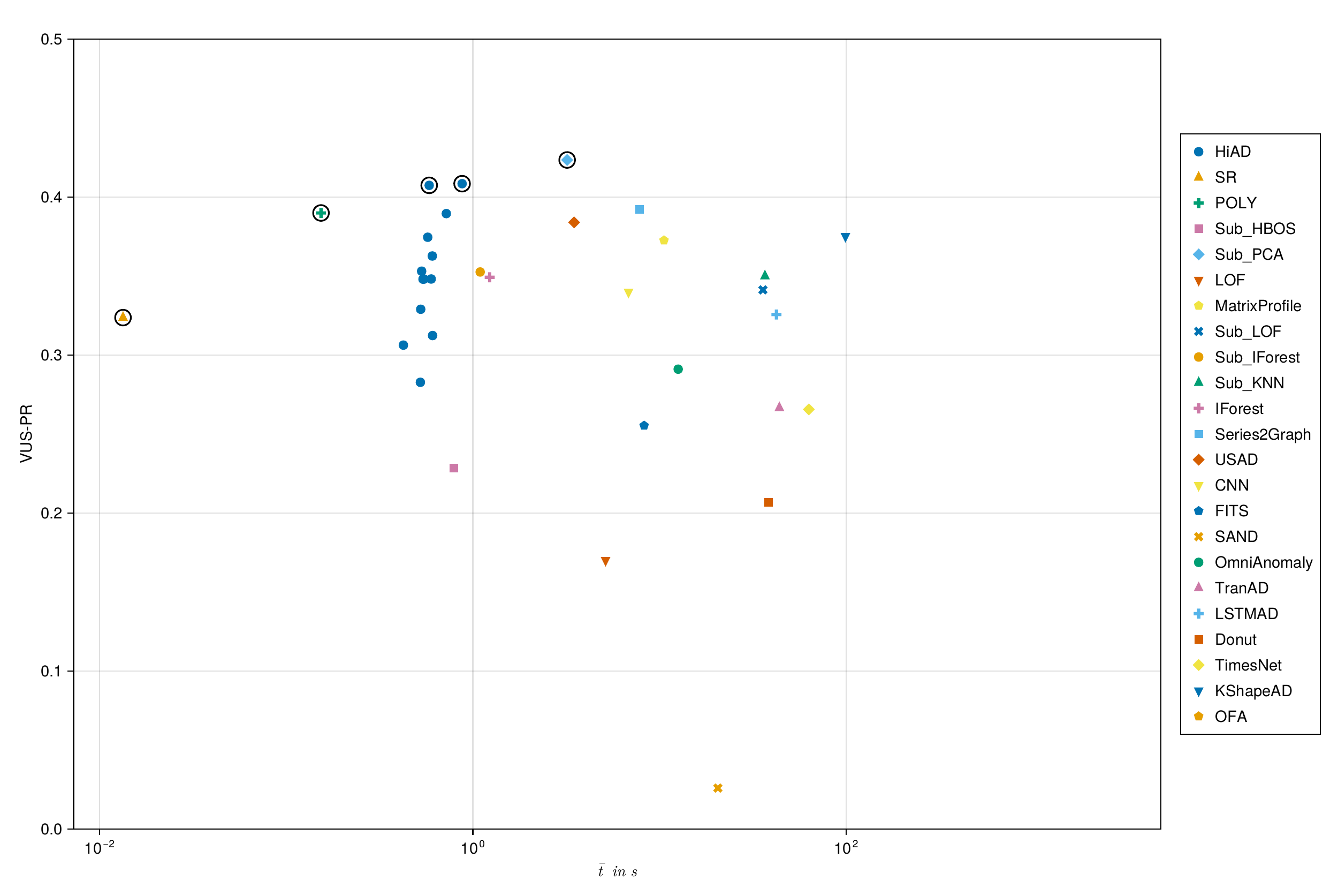
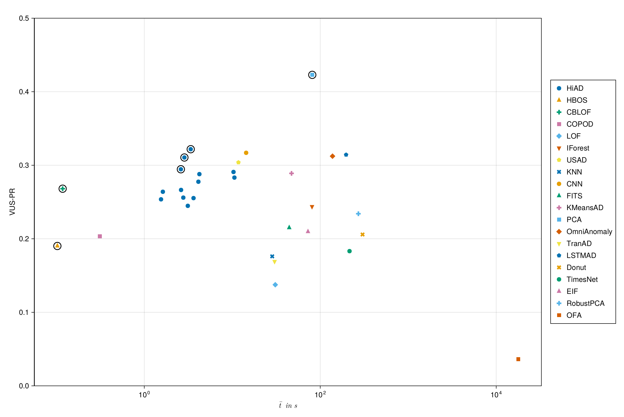
The most important result is not a single number — it’s a position in a two-dimensional space. The plots below show every method evaluated on the TSB-AD benchmark, plotted by average runtime against VUS-PR (a robust anomaly detection metric). Pareto-optimal methods are open-circles.
Show Document in new tab: hiad_pareto_frontier.html
HiAD sits on the Pareto frontier in both the univariate and multivariate settings. To beat its accuracy you pay substantially more in runtime — OmniAnomaly is 48× slower on the multivariate benchmark at an equivalent score. To beat its speed you give up substantial accuracy.
Expand for the figures from the paper, with method labels.
A real-world example: 12-lead ECG, with Noise
The poster shows a clean version of this figure.

Here it is with 30% missing data, and 5% dropped runs (50 samples missing at a time).
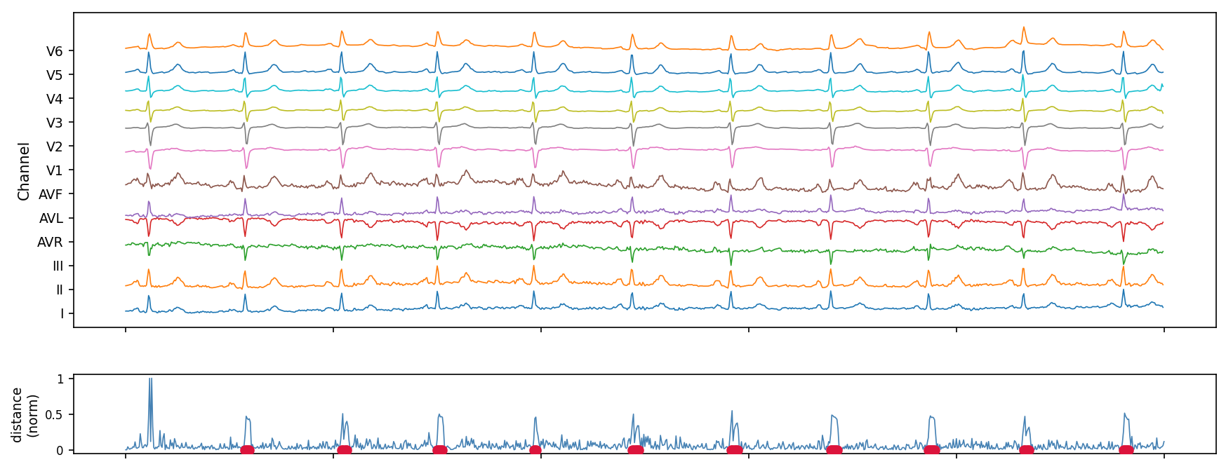
HiAD is run on a 12-lead ECG recording, all leads processed simultaneously as a 12-dimensional stream. The bottom panel shows the normalised internal distance measure over time, with detected anomalies marked in red. The distance trace is periodic — reflecting the regular QRS complex.
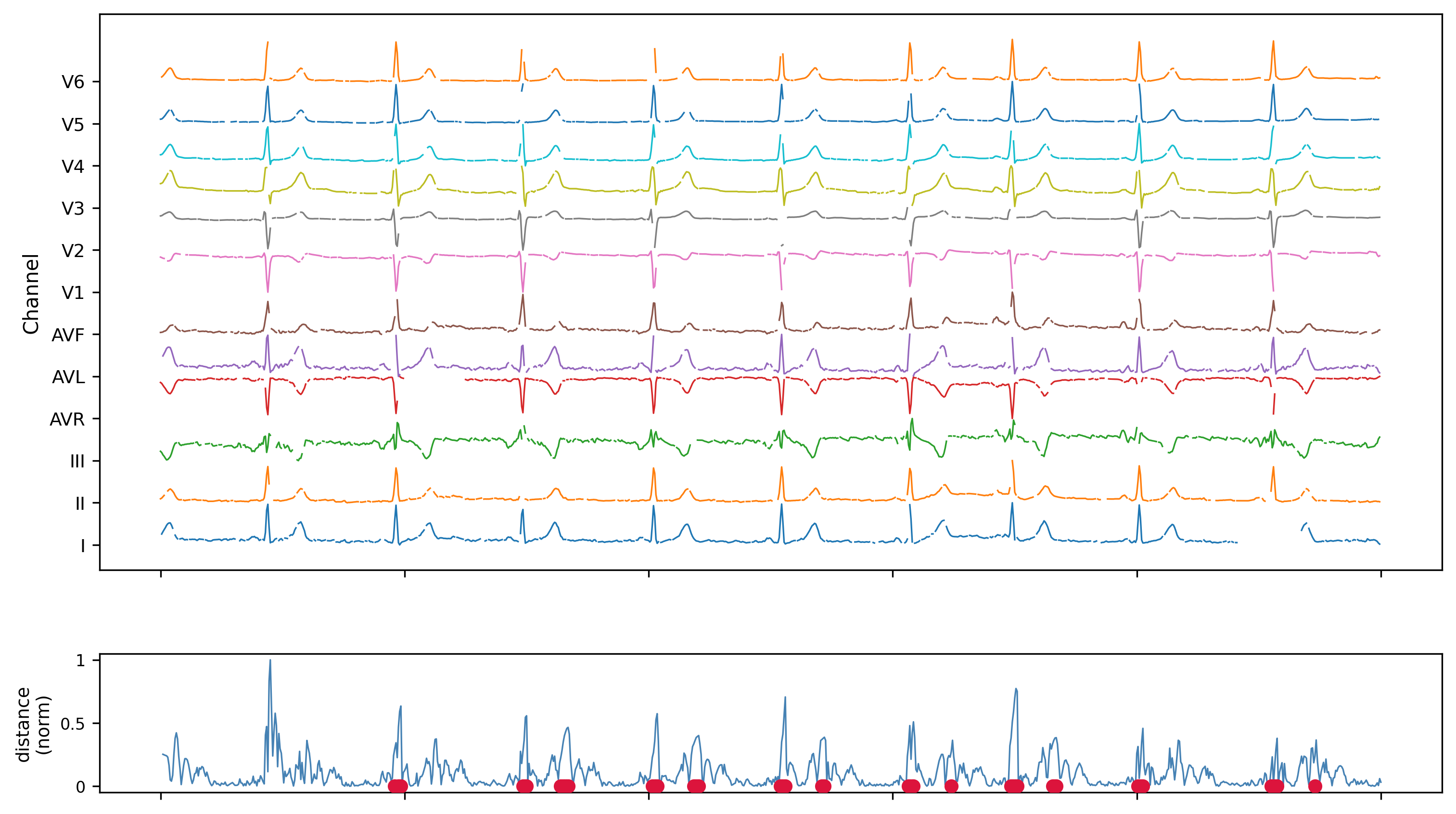
No resampling was needed across leads. No imputation was applied, neither was the ECG preprocessed in any way. The algorithm ran in a single pass with constant memory.
Missing data: a capability the poster couldn’t show
Real sensor networks are messy. Sensors drop out. Data arrives unevenly. The standard fix is imputation — fill the gaps before running detection. The problem is that common imputation strategies actively harm detection:
- Mean-filling suppresses the jolts in the HiPPO state that the detector relies on
- Zero-Order Hold introduces artificial transitions that look like anomalies to the algorithm
HiAD handles missing data natively. Each sensor has its own internal clock. If no observation arrives for a sensor at a given timestep, the clock simply doesn’t advance and the state isn’t updated. No imputation, no artifacts.
The figure below compares HiAD, windowed PCA, and CNN on a multivariate dataset with 50% of observations dropped at random and 5% sensor dropout with sequences up to 380 samples long. Panels from top to bottom: detection scores, the original full signal, the signal as HiAD sees it (with gaps), and the same signal after ZOH imputation (what PCA and CNN receive).
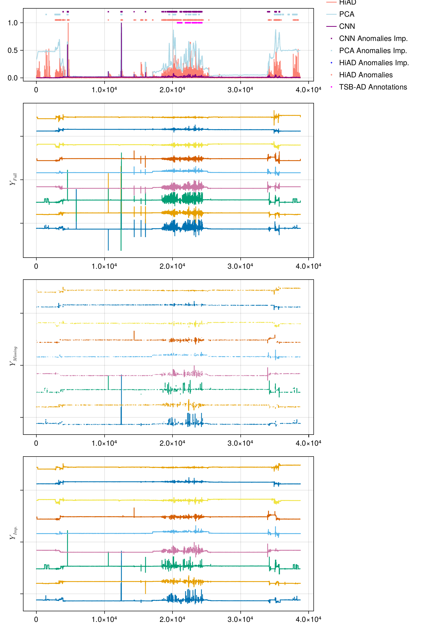
HiAD maintains qualitatively coherent detection throughout. PCA and CNN, which require imputation as a preprocessing step, degrade noticeably — the imputation itself introduces false positives.
Parameter guide
HiAD has several knobs, but it’s designed to be robust across reasonable settings. Here’s where to start:
| Parameter | Default | What it does |
|---|---|---|
| HiPPO method | LEGT | Sliding window over recent history. LEGS for longer memory, FOUT for oscillatory signals. |
| Order N | 8 | Polynomial expressiveness. Diminishing returns past 32. |
| Threshold α | 0.01 | Flags the top α fraction of distances as anomalous. |
| Influence β | 0.75 | How much anomalous inputs shift the internal state. Never set to 0 on non-stationary data. |
| Decay λ | 0.999 | How quickly old distance history is forgotten. Use 0.99 for fast-changing environments. |
| Histogram centers | 200–1000 | Resolution of the ECDF estimate. Below 200 is not recommended. |
The two parameter that matter most in practice are HiPPO method and β. If you mismatch the method with the data you observe it will likely perform a lot worse. Setting it to 0 tells the model to completely reject anomalous inputs from its state update — which sounds conservative but causes cascading false positives whenever the underlying signal drifts. The default of 0.75 is a good starting point for most settings.
What’s next
Several directions are actively being explored:
- Inter-sensor correlations. HiAD currently treats sensors independently. Incorporating a streaming covariance estimate (e.g. CCIPCA) would let it detect anomalies that manifest as correlation breakdowns rather than per-sensor deviations.
- Adaptive coefficient weighting. Lower-order HiPPO coefficients capture baseline trends, higher-order ones respond to transients. Reweighting them based on stream dynamics could improve discrimination without requiring a training phase.
- Multi-marginal ECDF scoring. Replacing the single scalar distance ECDF with one distribution per sensor dimension, combined in the spirit of ECOD, would be more robust at high dimensionality.
This method is currently under peer review. Code and full technical details will be shared upon publication.